TEXT: Introduction to NV centers in diamond and cavity-based magnetometry

1. NV centers in diamond

2. Microwave cavity

3. Coupling between NV centers and microwave cavity

1. NV centers in diamond

Watch the Youtube video below to learn how diamonds are valuable to quantum information science!

from IPython.display import IFrame
IFrame('https://www.youtube.com/embed/VCT0wDLyvSs', width=700, height=350)

For a comprehensive review of NV centers in diamond, you may also read over the slides in the download link below:

Click here to download.

1.1 Crystallographic structure

Diamond is a particularly interesting material in the realm of quantum information science. It is an excellent host substrate for optically active quantum emitters due to its wide bandgap (5.5 eV) and large transparency window. Among the many color centers in diamond, the negatively charged NV center is most famous for applications in quantum sensing and communication. It is a defect in the carbon lattice consisting of a substitional nitrogen atom accompanied by a vacancy site (see the left figure below).

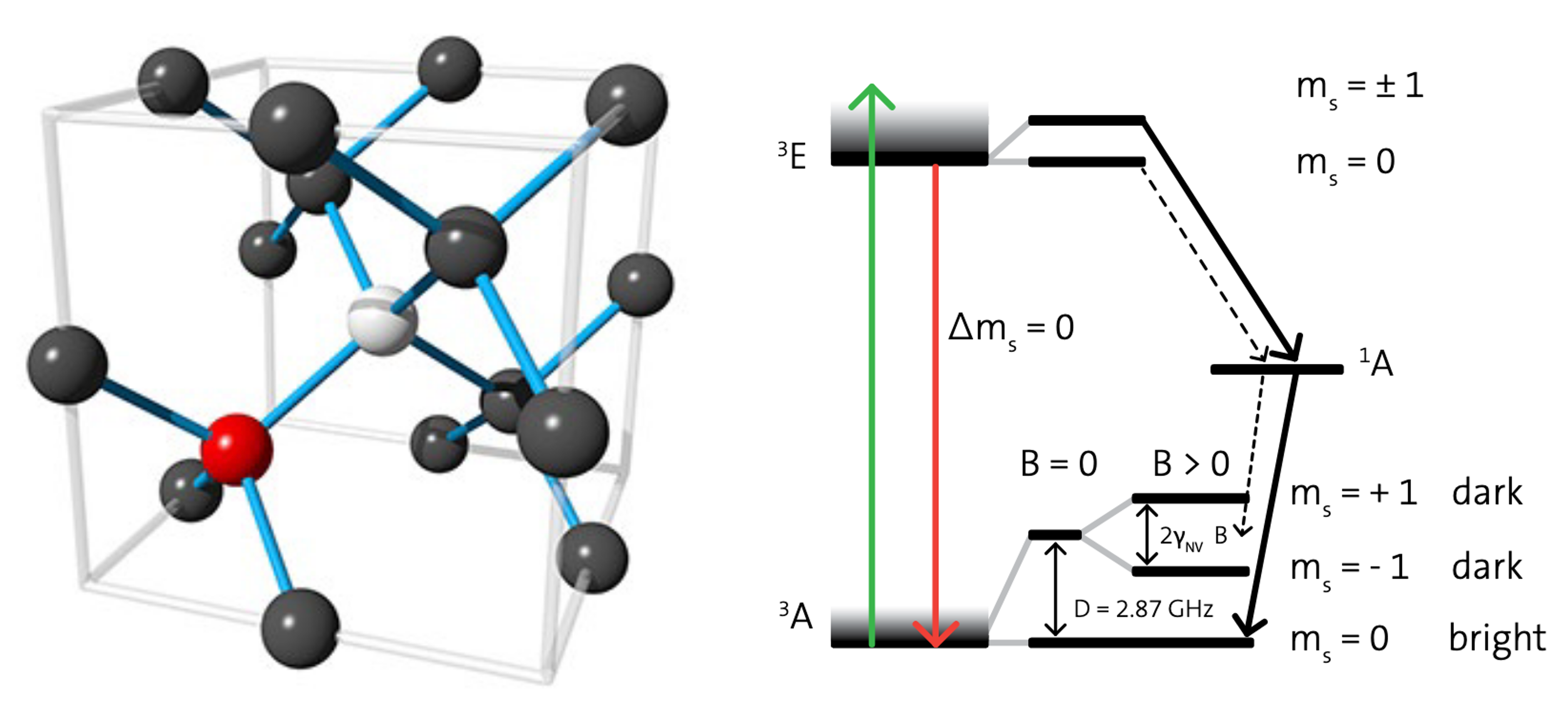
Fig. 49 Figures adapted from quTools, quNV brochure.

Effectively, NV center is an artificial atom in a solid state environment with well-defined optical transitions. More importantly, NV center’s spin states have energy splitting sensitive to the environment’s magnetic field strength. The greater the magnetic field strength, the greater the splitting. In a way, NV center itself is a magnetic field sensor. One can then readout the spin states (at microwave frequencies) to measure ambient magnetic field.

1.2 Level structure

Now we briefly go over the level structure for NV center. If you are not familiar with atomic level structures, fear not! It is simply a diagram that locates the relative locations of different energy states. The exact details are not important, but for pedagogical sakes, I will briefly walk through what the above right diagram is trying to show.

On the left-hand-side of the level structure, there are a ground state \(^3\)A and an excited state \(^3\)E. When the NV center decays from \(^3\)E to \(^3\)A, it emits a red photon at 637 nm. The reverse can also occur by shining the NV center with higher-energy (shorter wavelength) light at 532 nm such that it gets pumped from \(^3\)A to \(^3\)E.

Next, we delve further into the different pathways the NV center can go from \(^3\)A to \(^3\)E. Within \(^3\)A, there exist three hyperfine states: \(m_s=-1,0,+1\). Under zero magnetic field, the \(m_s=\pm 1\) states are degenerate, meaning they have the same energy. The difference in frequency between \(m_s=0\) and \(m_s=\pm 1\) is \(D=2.87\) GHz (caused by crystal field splitting). If the NV center begins at \(m_s=0\) and is excited to the excited state \(^3\)E via 532 nm pumping, there is a strong probability that it would decay back to \(m_s=0\) within \(^3\)A. However, if it begins at \(m_s=\pm 1\) and is excited to \(^3\)E, it is now more likely to undergo intersystem crossing, which is an another decay pathway that takes the NV center to a metastable \(^1\)A state. Afterwards, it would preferentially decay back to \(m_s=0\). Two crucial take-aways here. One, this intersystem crossing process does not emiter 637 nm photons. Second, it preferentially returns what is initially \(m_s=\pm 1\) to \(m_s=0\). Therefore, if you continuously pump the NV center with 532 nm light, in steady state, it would likely be in \(m_s=0\). This mechanism is called spin polarization.

Let’s consider this continuous pumping (spin polarization) case. We expect the fluorescence intensity, i.e. the number of emitted 637 nm photons, to be constant in steady state. However, when we apply a microwave drive at exactly 2.87 GHz, we start shuffling the state between \(m_s=0\) and \(m_s=\pm 1\) via Rabi oscillation. In this case, the fluorescence intensity would experience a dip. This phenomenon is called optically detected magnetic resonance (ODMR).

Fig. 50 Optical detected magnetic resonance. Figures adapted from quTools, quNV brochure.

Recall previously, we assume there is no applied magnetic field such that \(m_s=-1\) and \(m_s=+1\) states are degenerate. If we do apply magnetic field to the NV center, however, the degeneracy would be broken. \(m_s=-1\) and \(m_s=+1\) states would start splitting apart, and their energy difference grows linearly with the magnetic field strength due to the Zeeman effect. Now instead of 2.87 GHz, there would be two microwave frequencies at which the fluorescence intensity would experience a dip (can you see why?). Effectively, by detecting the optical signal coming from the NV center and noting where the changes in the intensity occur, we can extract information about the applied magnetic field. This means the NV center itself acts as a magnetometer!

HOWEVER, realistically, the change in fluorescence is quite minimal. To make a magnetometer that is practical, we will pursue an alternative approach in this lab. Instead of inferring information about the magnetic field through optical detection, we will attempt microwave detection.

2. Microwave cavity

2.1 Cavity mode of a cylindrical resonator

To do so, we need to first understand what a microwave cavity is and how it works. The cavity that we will be using in the experiment is a cylindrical resonator (you may also recall from your E&M class Chapter 8 in Classical Electrodynamics by J. D. Jackson). The resonator mode of interest is the so-called TE\(_{01\delta}\) mode, which has \(H_z,H_{\rho},\) and \(E_{\phi}\) components in cylindrical coordinates. Explicitly,

\[H_z = H_1 J_0(k_c\rho) f(\tilde{z})\]

\[H_{\rho} = -\frac{j\beta}{k_c} H_1 J_1(k_c\rho) f'(\tilde{z})\]

\[E_{\phi} = -\frac{j\omega\mu_0}{k_c} H_1 J_1(k_c\rho)f(\tilde{z})\]

where \(k_c=x_{01}/r_d\), where \(x_{01}\) is the first root of the Bessel function \(J_0(x)=0\) and \(r_d\) is the outer radius of the resonator. \(J_1\) is the Bessel function of the first kind of order 1. \(f(\tilde{z})\) is a factor that gives longitudinal dependence. If you are interested in its exact form, you may consult the Supplement of this paper.

Crucially, the \(H\) components imply that it is magnetic cavity, with the field profile shown in the figure below:

Fig. 51 Simulation results from Eisenach et al.

where the black dashed lines mark the outline of the resonator.

2.2 Cavity resonance frequency

The resonance frequency \(\omega_c\) can be calculated by solving the coupled equations:

\[\zeta \tan\left(\frac{\zeta L}{2}\right) = \zeta_0\]

\[\zeta = \sqrt{\epsilon_r \frac{\omega_c^2}{c^2}-\frac{x_{01}^2}{r_d^2}}\]

\[\zeta_0 = \sqrt{\frac{x_{01}^2}{r_d^2}-\frac{\omega_c^2}{c^2}}\]

where \(\epsilon_r\) is the relative dielectric constant and \(x_{01}\) is again the first root of the Bessel function \(J_0(x)=0\). \(L\) is the length of the resonator.

For more details on the derivation, you may consult this paper or the previous cylindrical resonator reference.

2.3 Inductive coupling between a microwave cavity and a loop coupler

From our beloved right-hand rule, you may know that the magnetic field should follow the black arrows in the figure below:

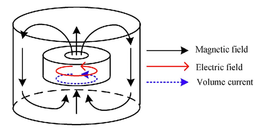
Fig. 52 Field components of a cylindrical microwave cavity.

How do we experimentally measure the cavity resonance? It’s simple! We can simply use a metallic loop that inductively couples to the magnetic cavity. As such, we call it a loop coupler. The magnetic field exiting out of the cavity in the \(z\) direction (pointing up shown in the figure above) threads through the loop coupler, thereby inducing a current that is measurable. We will leverage this fact and read out the cavity resonance via a vector network analyzer (VNA), which you should have already gotten familiar with during the Parkour session.

2.4 Quality factor

One important metric to the quality of a microwave cavity is its quality factor, which is defined as:

\[Q = \omega_d/\kappa_c\]

where \(\kappa_c\) is the total cavity decay rate (in units of radian-frequency). The higher the \(Q\), the longer the electric field is “trapped” inside the cavity. Since \(\kappa_c\) is inversely proportional to \(Q\), higher \(Q\) also corresponds to narrower cavity resonance feature (a dip in reflection for our case) in frequency.

A cavity’s \(Q\) is also the geometric mean of its intrinsic quality factor \(Q_0\) and quality factors due to leakage. For an instance, if we bring a loop coupler near the microwave cavity, we are artificially introducing a channel into which the energy of the cavity mode can escape. In this case, the loop coupler is a leakage source and introduces its own “quality factor”, \(Q_1\). Hence,

\[\frac{1}{Q} = \frac{1}{Q_0}+\frac{1}{Q_1}\]

Conventionally, when we purposefully introduce a leakage channel, we call the cavity \(Q\) the loaded quality factor.

It is also often easier to consider in terms of decay rates. We can rewrite the above expression as

\[\kappa_c = \kappa_{c0}+\kappa_{c1}\]

where \(\kappa_{c0}\) is the intrinsic cavity loss rate and \(\kappa_{c1}\) is the additional decay rate into the loop coupler.

3. Coupling between NV centers and microwave cavity

So far, we have discussed two distinct entities, NV centers in diamond and microwave cavity. In our experiment, we will combine the two systems by simply putting a diamond sample full of NV centers inside the microwave resonator. There are two conditions we must first satisfy in order to observe quantum sensing with solid state spins. One, we need to first excite the entire diamond with 532 nm light, hence spin polarizing an ensemble of NV centers. Second, we need to apply the appropriate amount of magnetic field to shift the energy level of \(m_s=+1\), such that the frequency difference between \(m_s=+1\) and \(m_s=0\) matches the resonance frequency of the microwave resonator. When the aforementioned conditions are met, we can observe the quantum mechanical response of the coupled system (consisted of NV centers and microwave cavity) by sending a microwave signal and measuring its reflection coefficient. Experimentally, we will have the VNA send microwave pulses across different frequencies down the loop coupler, which returns reflected pulses from the microwave cavity back to the receiving port of the VNA.

The reflection coefficient \(\Gamma\) is given by:

\[\Gamma = -1+\frac{\kappa_{c1}}{\frac{\kappa_c}{2}+j(\omega-\omega_c)+\frac{g^2}{\frac{\kappa_s}{2}+j(\omega-\omega_s)+\alpha}}\]

where \(\kappa_c=\kappa_{c0}+\kappa_{c1}\) is the sum of the unloaded (intrinsic) and input port (loop coupler) loss rates, respectively. \(\kappa_s=2/T_2\) is the homogeneous width of the spin resonance where \(T_2\) is the coherence time. \(\alpha\) captures the effect of saturation and is beyond the scope of this introductory discussion. \(g\) is the effective coupling strength between the NV centers and the cavity mode. \(\omega\) and \(\omega_s\) are the probe (sent out of the VNA) and the spin resonance frequencies, respectively. Since there are parameters regarding the NV centers themselves, the quality of the diamond indeed affects the reflection contrast. You will explore different types of diamond in this lab.

For those who are interested in deriving the reflection coefficient formulae (via input-output formalism similar to the case in quantum optics), you may consult this paper.

Here we compare the conventional ODMR result (optical-based) and the introduced microwave cavity-based approach by showing you experimental results by Eisenach et al.:

Fig. 53 ODMR and microwave readout results from Eisenach et al.

Due to coupling with the cavity, the NV centers’ microwave response (blue) exhibits much greater signal-to-noise ratio (SNR) than conventional ODMR (red)!

In the first portion of the lab, you will use the given formulae for the reflection coefficient and assess how each parameter affects the NV centers’ microwave response.

Pre-Lab Questions

In the first session of this experiment, you will first be characterizing the microwave cavities by measuring their resonance frequencies and quality factors. Recall that a cavity \(Q\) is defined to be the ratio of its resonance frequency to its decay rate (also known as the cavity linewidth).

1. Calculate the \(Q\) of a cavity with resonance frequency at 3 GHz and linewidth of 100 kHz.

2. Typically the cavity linewidth is defined at the full width at half maximum. Insert a cell below and write a Python script plotting a resonance peak centered at 3 GHz with linewidth of 100 kHz. Make the x-axis frequency with a span of 1 MHz and the y-axis normalized cavity transmission. Note that the cavity lineshape is usually Lorentzian.

The second part involves characterizing the Helmholtz coil by measuring its generated magnetic field. Recall that due to the Zeeman effect, magnetic field is used to shift the energy (frequency) difference between the \(m_s=0\) and \(m_s=+1\) states of NV centers. Importantly, the correct amount of magnetic field must be applied to ensure the energy difference matches the microwave cavity’s resonance frequency.

3. The amount of frequency shift due to magnetic field strength \(B\) is \(\delta f = \mu B\), where \(\mu = \mu_B g/h\). \(\mu_B\) is the Bohr magneton, \(g\approx 2\) is the Lande factor, and \(h\) is the Planck constant. Calculate \(\mu\) in units of MHz/Gauss. Note the SI unit for magnetic field is Tesla, where 1 Tesla = \(10^4\) Gauss.

4. Calculate the needed magnetic field strength (in Gauss) if the cavity resonance frequency is at 3 GHz. Recall the starting point (due to crystal field splitting) of the energy difference between \(m_s=0\) and \(m_s=+1\) is 2.87 GHz.