LAB – Hanbury Brown - Twiss Lab (Week 1)

LAB – Hanbury Brown - Twiss Lab (Week 1)#

Introduction#

In this lab we’re going to perform the Hanbury Brown - Twiss (HBT) experiment with the quED set-up. We want to perform the measurements and also understand what they mean in terms of the calculations. This entire lab will take less than 2 sessions of the course, and it will help prepare you for performing the QKD protocol over the following 2 sessions.

This write-up will cover a few topics:

Lab Goals are your guidance for what this experiment will accomplish. Your write-up should address all of these.
Coincidence Estimate is an important calculation to do so you can make sure you’re measuring what you expect. It will also be an example of relating a measured experimental to a theoretical calculation.
quED power up describes how to turn on the quED to begin taking data.
Experimental set-up: 2-fold gives an overview on how to perform the 2-fold experiment. There is a Python cell for you to input your experimental measurements and find \(g^{(2)}(0)\)
Experimental set-up: 3-fold gives an overview on how to perform the 3-fold experiment. There is a Python cell for you to input your experimental measurements and find \(g^{(2)}(0)\)

We’ll be following the quTools manual, which you can find online here: https://www.qutools.com/files/quED/quED-HBT/quED-HBT-manual.pdf

Goals for this lab#

In this lab, we have a few goals:

Measure \(g^{(2)}(0)\) for the SPDC output in the heralded and un-heralded regimes. You will need to take enough points to find both an average and a standard deviation. How did you choose which integration time to use?
Compare \(g^{(2)}(0)\) measurements for different pump laser currents: 10 mA, 25 mA, and 40 mA. Again, make sure you take enough data points to find the variance.
Compare your experimental results with what you calculated. How did your calculations match your measurements? Why do you think they were different?
Use the \(g^{(2)}(0)\) measurements to categorize when the SPDC output counts as a single photon source. Consider whether you would classify the light source as being in a number state, coherent state, or thermal state.

Keep in mind that you will need to address all of these points above in your 2-3 page write-up at the end of this T2E1 lab sequence. It is then important we address these issues properly during lab time. Also remember that everyone is expected to keep notes during the lab, and you should include collected data, code, and analysis in those notes. The instructions you’re reading right now are meant to guide you through taking the data and looking at some of the data analysis.

Estimate coincidence count for uncorrelated sources#

If I said I have two sources of light that are totally independent, what would you estimate the coincidences to be? You have access to the following values:

The singles count of each source of light (read off the quCR)
The coincidence window (30 ns)
Integration time (set on quCR)

Use the next cell to evaluate your estimate of coincidents.

import numpy as np

S1 = 5E4 # units cps
S2 = 5E4 # units cps
cw = 30E-9 # set by qutools as 30 ns
inttime = 1 # default to 1 second

def accidentals(S1,S2,cw,inttime):
    it = -1
    
    return it

it = accidentals(S1,S2,cw,inttime)

'Coincidences: {:.3e} with singles {:.3e} and {:.3e} after {:.1f} seconds'.format(it, S1, S2, inttime)

'Coincidences: -1.000e+00 with singles 5.000e+04 and 5.000e+04 after 1.0 seconds'

Does your estimate match what you see? You can use the light collected from the overhead lamps as uncorrelated light.

quED power up#

If the screen is dark on the quED, flip the plastic switch on the bottom left corner of the front panel.

To turn on the laser, verify that the set current is 0 mA. Then press the button to the right of the screen on the front panel. It will light up when the laser is active.

Now, verify the laser is in CW mode and turn the pump current to 35 - 40 mA.

Next, check the singles counts. You should see about 100,000 cps from the signal and the idler. The coincidence counts should be on the order of 5,000 to 10,000.

Troubleshooting low counts#

If you see fewer counts - say 20% below the maximum - try adjusting the mounts with the lenses that collect the SPDC output light into fibers.

If that doesn’t work or you see severely reduced counts, try walking the beam using the mounts with the mirrors. If this is your first time aligning the quED this way, ask an instructor to help.

If that doesn’t work, ask an instructor to show you the full alignment procedure. You’ll use a fiber fault finder to back propagate into the box with the source.

HBT with 2-fold coincidence#

Recall that the HBT experiment has the follow schematic:

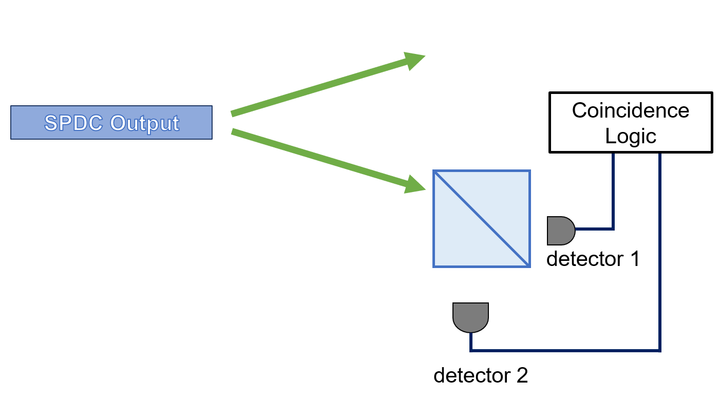
_images/HBT_lab.png — Fig. 45 Setup for HBT measurement.#

We want to set that up with the quED. quTools provides the following cartoon:

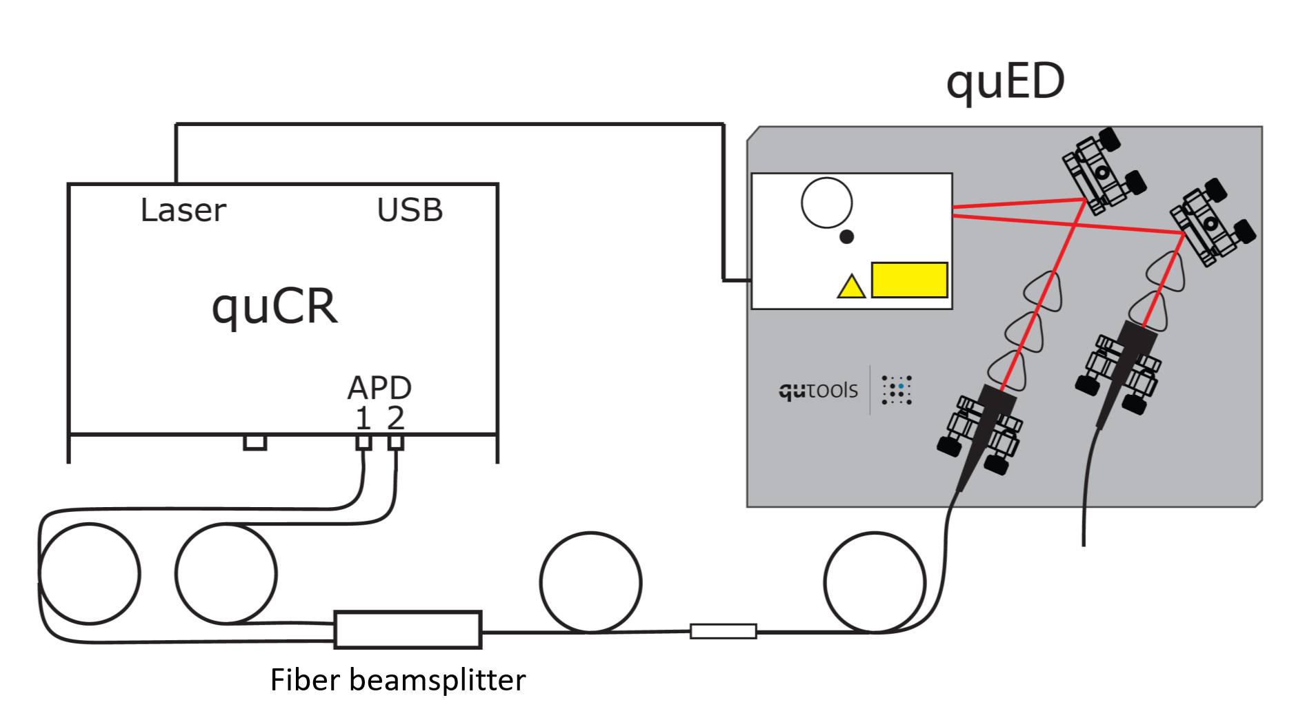
_images/HBT_lab_qutools.png — Fig. 46 Image from quTools of the HBT experiment with quED#

You can read off the singles and coincidences from the quED detection page directly. The detection page will scroll through a time plot, the settings page, and another page that will display a numerical value for the singles and coincidences after each integration time. You can also use the Python wrapper function to read the detected values directly from the quED.

Calculating \(g^{(2)}(0)\) from experimental data#

Recall that the equation for \(g^{(2)}(0)\) is

\[g^{(2)}(0) = \frac{\langle\hat{n}_1\hat{n}_2\rangle}{\langle\hat{n}_1\rangle\langle\hat{n}_2\rangle}\]

You’ll note that this equation has nothing to do with the coincidence window \(\Delta_w\), but consider the following thought experiment. Keeping integration time \(T\) constant, you look at coincidences \(\langle\hat{n}_1\hat{n}_2\rangle\) using an infinitely long coincidence window and then you perform the same measurement at an infinitely small but still nonzero coincidence window. Do you expect to see more coincidences on the long or short window? Thus, coincidence windows do matter in terms of scaling for \(g^{(2)}(0)\).

For this reason, we want to look at the calculation in a slightly different way. Specifically, consider that the calculation asks for the expected value of the coincidences and singles. What we measure are the rates, \(R_i\) of the singles and coincidences, expressed in counts per second (cps). That means that to find a probability, \(p_i\), within a given coincidence time, \(\Delta_w\), we need to consider

\[p_i = R_i\Delta_w\]

We can consider the cases were \(i\) refers to \(1\), \(2\), and \(12\), so if we want to look at the expected value in terms of the measured values, we want to evaluate

\[g^{(2)}(0) = \frac{R_{12}}{R_1R_2\Delta_w}\]

The next cell is provided for you to input your own code to calculate \(g^{(2)}(0)\) from your experimental values.

# Use this cell to plug in your measured data and get a value for g2

S1 = 5E4 # singles in detector 1 - cps
S2 = 5E4 # singles in detector 2 - cps
cw = 30E-9 # coincidence window set by qutools as 30 ns

coincidences = 10 # coincidences between 1 and 2 per second
inttime = 1 # integrationd time: default to 1 second

def g2twofold(S1,S2,cw, coincidences, inttime):
    it = -5
    
    return it

it = g2twofold(S1,S2,cw, coincidences, inttime)

'G2: {:.3e} with coincidences {:.3e}; singles {:.3e} and {:.3e} after {:.1f} seconds'.format(it, coincidences, S1, S2, inttime)

'G2: -5.000e+00 with coincidences 1.000e+01; singles 5.000e+04 and 5.000e+04 after 1.0 seconds'

Remember to take enough measurements to find the average and the standard deviation. Also, look at the effect of changing the integration time and comment in your write-up about how that affects the calculated \(g^{(2)}(0)\). How does \(g^{(2)}(0)\) change with different pump currents? Would you describe this configuration as a single photon source?

HBT for heralded source (3-fold coincidence)#

As you recall, we want to modify the HBT experiment to look at the HBT experiment with a heralded single photon source, as shown below.

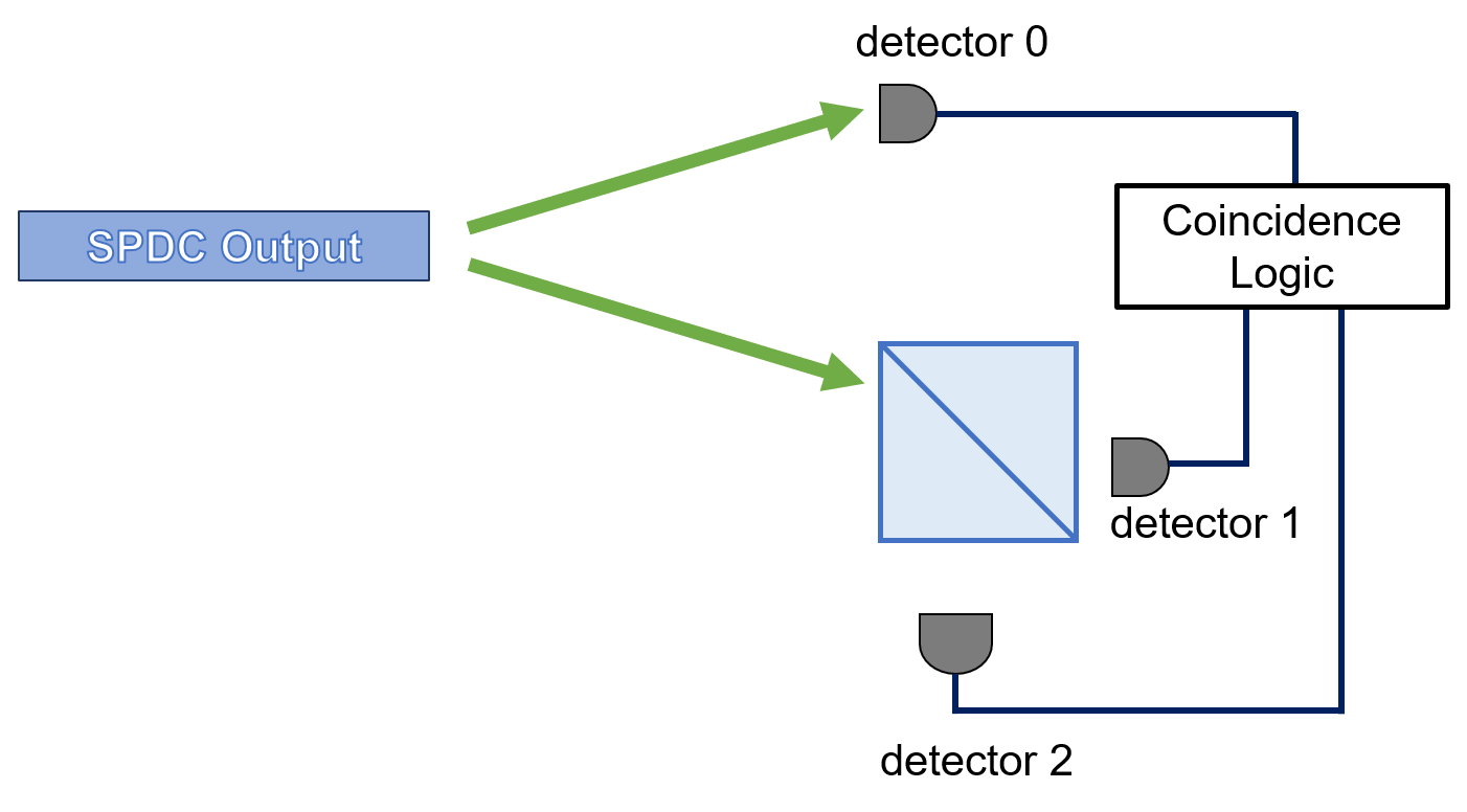
_images/HBT_heralded_lab.png — Fig. 47 Setup for heralded HBT measurement.#

quTools provides a more detailed schematic of how this experiment will look with the quED.

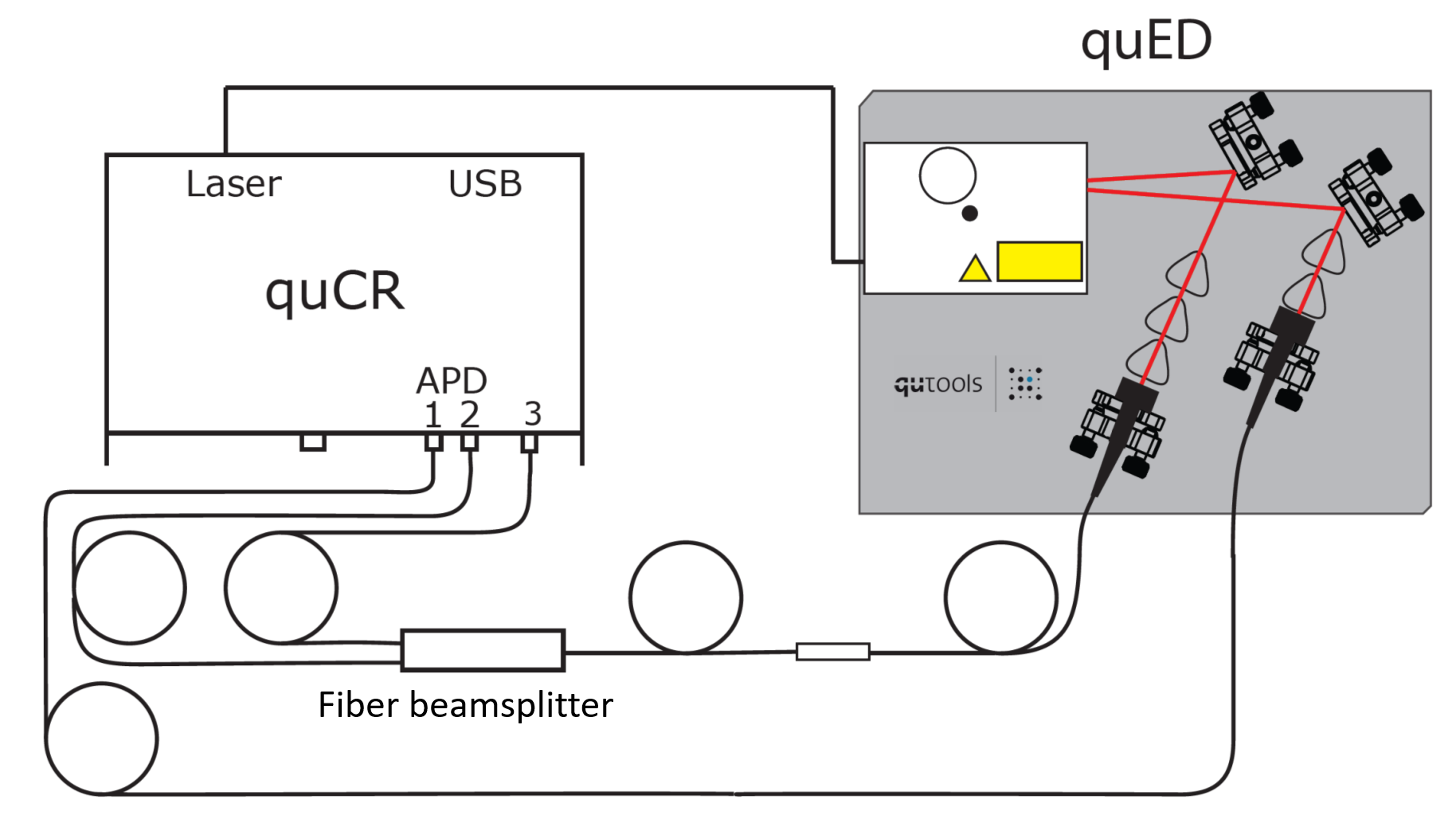
_images/HBT_heralded_lab_qutools.png — Fig. 48 Image from quTools of the HBT experiment with heralded source with quED#

You can use the equation from the text to find \(g^{(2)}(0)\) for the heralded source:

\[g^{(2)}(0) = \frac{N_{012}N_0}{N_{01}N_{02}}\]

Again, the next cell is provided for you to input your own code so you can caluclate your \(g^{(2)}(0)\) as you collect data.

# Use this cell to plug in your measured data and get a value for g2

N012 = 1E5 # 3-fold coincidences
N0 = 5E4 # singles in detector 0 - cps
N01 = 5E4 # 2-fold coincidences
N02 = 30E-9 # 2-fold coincidences


inttime = 1 # integrationd time: default to 1 second

def g2threefold(N012,N0,N01,N02,inttime):
    it = -0.5
    
    return it

it = g2threefold(N012,N0,N01,N02,inttime)

'G2: {:.3e}'.format(it)

'G2: -5.000e-01'

Again, don’t forget to explore how \(g^{(2)}(0)\) changes when you change your pump current. Remember to see how integration time affects your measurements, and find the mean and standard deviation.