LAB – Quantum Sensing With Solid State Spins (Week 2)

LAB – Quantum Sensing With Solid State Spins (Week 2)#

Aim 3: Achieve strong coupling between NV centers and the microwave resonator#

Prelab#

Laser safety#

In this week, you will be running experiments with a free-space 532nm laser that goes up to 3W. Given that this is a class 4 laser, you must first undergo proper laser safety training.

In addition to the training session conducted by MIT EHS, we strongly urge you to read through the Laser Safety page here.

The teaching staff will also supply laser safety glasses (LG12 from Thorlabs with OD7 at 532\(~\)nm). You must be wearing these during the alignment step (step ii in Lab Exercise below) and during the experimental sequence (step vii).

If you have any questions or concerns regarding laser safety, do not hesitate to reach out to the teaching staff and MIT EHS (contact Judith Reilly, jmreilly@mit.edu).

Simulation with hyperfine transitions#

In the previous session, you were able to simulate avoided crossing for a single hyperfine transition. Since NV centers in the diamond(s) that you will be using in the Lab Exercise parimarily constitute N-14 isotope, which is spin-1, you should expect to see 3 hyperfine transitions.

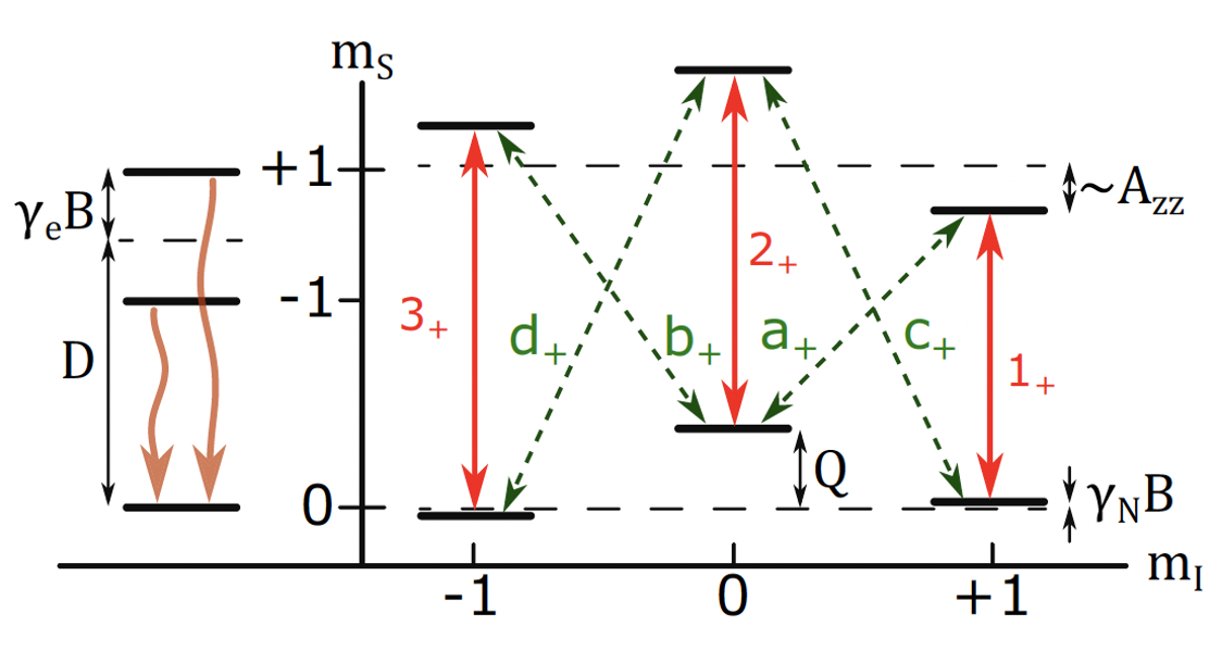
../_images/hyperfine_transitions.png — Fig. 59 Ground-state energy level structure of a single NV center. Left: electron spin levels. The solid black arrow depicts optical electron spin polarization to the \(m_S\) = 0 state. Right: coupled electron-nuclear spin levels in the \(|m_S\rangle\) = +1 electronic spin state. Solid red arrows show nuclear spin preserving transitions (\(1_+, 2_+\), and \(3_+\)). Dashed green arrows show nuclear spin exchanging transitions (\(a_+, b_+, c_+,\) and \(d_+\)). Figure adapted from Huillery et al..#

Please write a Python script that shows the 2D reflection spectra for 3 hyperfine transitions, spaced 2 MHz apart.

### Your code goes here

Lab Exercise#

i) Interface with the power supply#

Similar to interfacing with the VNA during T3E3-TRAINING, you will also need to be able to control the power supply via Python. First, install the packages qcodes, qcodes_contrib_drivers, and pyserial. Then, connect the power supply’s USB port to the laptop. Run the following cell to determine which serial port it occupies.

import serial.tools.list_ports
print(list(serial.tools.list_ports.comports()))

---------------------------------------------------------------------------
ModuleNotFoundError                       Traceback (most recent call last)
Cell In[2], line 1
----> 1 import serial.tools.list_ports
      2 print(list(serial.tools.list_ports.comports()))

ModuleNotFoundError: No module named 'serial'

Alternatively, you can also run python -m serial.tools.list_ports directly in terminal.

Following the example shown here, make sure you can set Channel 1’s voltage and turn Channel 1’s output on/off via Python commands.

### Your code goes here

ii) Aligning the laser to excite the diamond#

Inside the magnetic shield, there should be a 3D printed component with a thick microscope glass slide (square-ish).

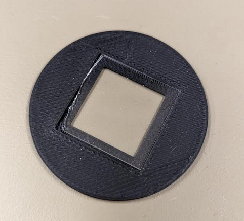
../_images/week2_3d_printed_mount.png — Fig. 60 3D-printed mount for diamond samples.#

Place a purple diamond on the glass slide close to the center. At this point, call your TA over to the station to turn on the laser (heavily attenuated such that the optical power is much less than 3 W). Please wear proper laser safety glasses now.

A 561\(~\)nm optical longpass filter will be placed to contain the 532\(~\)nm laser light. Your TA will then align the laser light to ensure it is incident on the diamond by turning the knobs of the 45-degree mirror at the bottom of the cage (see picture below).

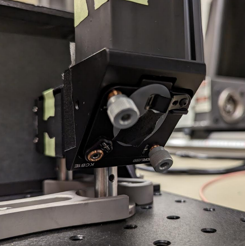
../_images/week2_mirror_knobs.png — Fig. 61 The 45-degree kinematic mirror mount with two knobs used for aligning the laser beam with respect to the diamond samples.#

Upon incidence, still with your laser safety glasses on, you should be able to see fluorescence emanating from the diamond. The fluorescence stems from the atomic transitions between the ground and excited states of the triplet manifold \(^3 E \leftrightarrow ^3 A\) in NV centers’ level structure. Recall from T3E3-TEXT that the direct emission from the exited state to the ground state corresponds to 637\(~\)nm. If instead of a 561\(~\)nm longpass filter, we have a 638\(~\)nm optical longpass filter in place. Will you still be able to observe fluorescence? Why or why not? You may find the photoluminescence spectrum below helpful.

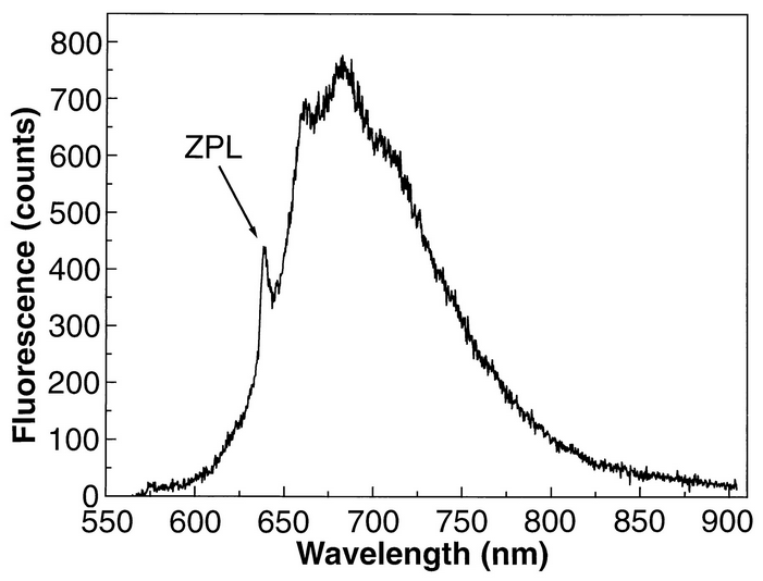
../_images/week2_nv_spectrum.png — Fig. 62 NV center’s photoluminescence spectrum. Figure adapted froom Gruber *et al.*.#

Now, the TA will turn off the laser and remove the longpass filter. Put the purple diamond back inside its original container. Again, with the pair of tweezers, grab the non-purple diamond and place it on the glass slide close to the center. Ask the TA to put the longpass filter back on top of the magnetic shield and turn on the laser again. Please make sure again you are wearing proper laser safety glasses. The TA will once again align the laser light to be incident on the diamond. Are you able to observe any fluorescence? Explain why or why not?

The TA will turn off the laser once again.

iii) Stack everything together!#

Recall from Aim 1, you had to stack the microwave resonators inside the magnetic shield. This time, you will stack even more things with your now seasoned tweezer skills.

The diagram shown below is a reference to what you will be stacking:

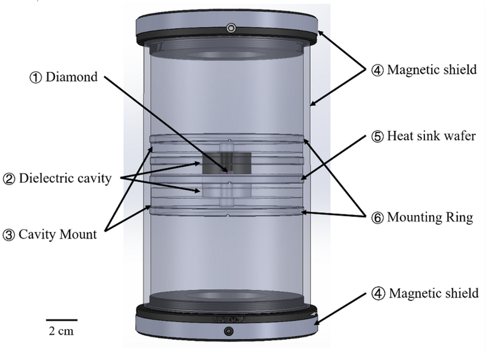
../_images/week2_stack.png — Fig. 63 Diagram depicting a combined stack of the magnetic resonators and a diamond sample placed inside a magnetic shield.#

You need to first remove the 3D printed component with the glass slide, and replace it with a custom-machined PTFE (Teflon) disk on the retaining ring inside the magnetic shield. Then, place one of the resonators (let’s call it resonator 1) on top of the PTFE disk, which should have a divet that (sort of) fits the microwave cavity. Next, put a thin microscope slide on top of resonator 1 in place of the “heat sink wafer”.

Put the other resonator (call it resonator 2) on top of the thin glass slide. Try to align resonator 2 to resonator 1 laterally.

Finally, use the pair of tweezers and “drop” the diamond inside resonator 2 (central hole). You should have the diamond standing on its thin side that is 0.5\(~\)mm thick. A good trick is to use the tweezers to nudge it to a standing position after dropping it into resonator 2. See the picture below for reference. Let the TA know if you are having troubles.

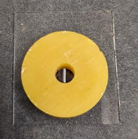
../_images/week2_diamond_in_cavity.png — Fig. 64 Example of a microwave cavity with diamond samples placed inside, each diamond standing vertically on its thin side (0.5\(~\)mm).#

iv) Realign the laser to excite the diamond#

We will now repeat step (ii). Let the TA know you are ready to turn on the laser and align the laser beam for you. Again, please wear your laser safety glasses now. This time, the attenuated laser beam is incident on the diamond through the holes of the resonators. You should still be able to “see” fluorescence from NV centers.

v) Optimize the position of the loop coupler#

In order to see avoided-crossing, you want to maximize the effective cooperativity of the spin-cavity system. The cooperativity \(C\) scales with \(1/\kappa_c\). In other words, we must ensure the quality factor is as high as possible, while keeping the loop coupler sufficiently close to be able to probe to cavity’s frequency response. Do your best to optimize the position of the loop coupler by changing its \(z\) coordinate to achieve the highest quality factor, i.e. smallest cavity linewidth. Unfortunately, its \(x,y\) positions will be fixed by the iris, which is intended as both an additional magnetic shield and laser block. Hence, you may need to adjust the tilt slightly in addition to \(z\).

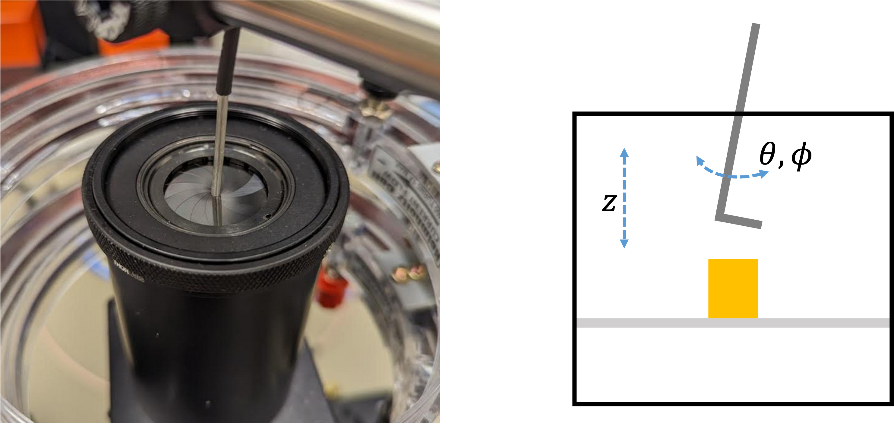
../_images/week2_iris_adjust.png — Fig. 65 (left) Picture of an iris wrapping around the looper coupler. (right) Diagram showing the degrees of freedom for optimizing the loop coupler’s position.#

Be sure to avoid knocking over the resonator stack with the diamond that you have carefully constructed while optimizing the loop coupler’s position.

vi) Write an experimental sequence to produce a 2D map of frequency vs magnetic field#

From T3E3-TRAINING, you were able to interface with the VNA via Python. And from part (i), you were able to interface with the power supply, which effectively drives the Helmholtz coil and thereby the amount of the mangetic field being generated.

Below, please write an experiment sequence that performs a 2D sweep over both frequency and magnetic field. The sweep over frequency is essentially done for you by the VNA. Your task here will be to grab a trace off the VNA (with carefully defined frequency center and span corresponding to the cavity signal), and sweep over a range of voltages. The voltage range, i.e. the sweeping range of the magnetic field strength, should cover the required field strength to shift the NV centers’ resonance to match the cavity resonance. This was calculated by you in Aim 1’s Prelab.

Importantly, for each magnetic field strength, you should obtain an average of a frequency trace. In your script, please also compute the variance of each point.

You should run a pseudo-experiment without the laser on to make sure the experimental sequence runs smoothly. Please also check that you can generate a 2D map of your acquired “data”.

### Your code goes here

vii) Run the experimental sequence and determine if you have achieved strong coupling#

Now, it is time to reproduce the avoided-crossing data you have seen in the demo and in your simulation results from Aim 2!

Call your TA over when you have reached this step. Remeber to put on your laser safety glasses. After your TA closes the iris (if you have not done so already) and places the foam (an additional laser block) above it, the laser will be turned on to its max power. At this point, run the experimental sequence you have scripted.

If the cavity quality factor is narrow enough, and the coupling strength between NV centers and the microwave resonator is sufficiently strong, the spin-cavity system should achieve strong coupling. In this case, your 2D map should contain “kinks” at each of the three hyperfine transitions.

If you are having troubles, discuss with your teammates about ways to increase the coupling strength, SNR, …etc. Consult with your TA afterwards.

Once you have obtained data exhibiting strong coupling, try increasing the number of VNA traces being averaged over per each magnetic field strength to see if the contrast improves further.

viii) Estimate the sensitivity#

With your acquired data, please estimate the maximal magnetic field sensitivity you have achieved. The phase noise of the spectrum analyzer in the VNA is measured to be -103\(~\)dBc/Hz at 1\(~\)GHz (for simplicity, we will assume the noise level is the same for our frequencies).

You should:

First, convert the phase noise \(d\phi\) to \(V_{\text{rms}}/\sqrt{\text{Hz}}\). For this, you will need to obtain the input power from either the libreVNA GUI or use the Python interface.
Second, re-plot the 2D data for \(dV/dB\), where \(B\) is the magnetic field strength and \(V\) is the r.m.s. voltage \(V_{\text{rms}}\). Note that the data you extract from the VNA via Python is in dBm (power).
Third, find the maximum \(dV/dB\) and compute \(d\phi/(dV/dB)_{\text{max}}\) in pT/\(\sqrt{\text{Hz}}\). This would be your maximum magnetic field sensitivity, assuming your noise floor is limited mainly by the VNA’s phase noise.