EXTRAS – Rigorous Solution of Mach-Zender Interferometer

In the course material for the discussion of single-photon interference and the interaction-free measurement, we took a shortcut to calculating the photon number expectation by ignoring the operators of the vacuum state inputs. This simplifies the problem, but is not a rigorous solution. A particular shortcoming is that this approach would give incorrect results for calculating the noise properties of the photon number at the detectors as in that case the vacuum state input does matter.

Complete solution without an object

The problem setup is the same, however now we must include all inputs, which slightly modifies our setup as shown in Fig. 28.

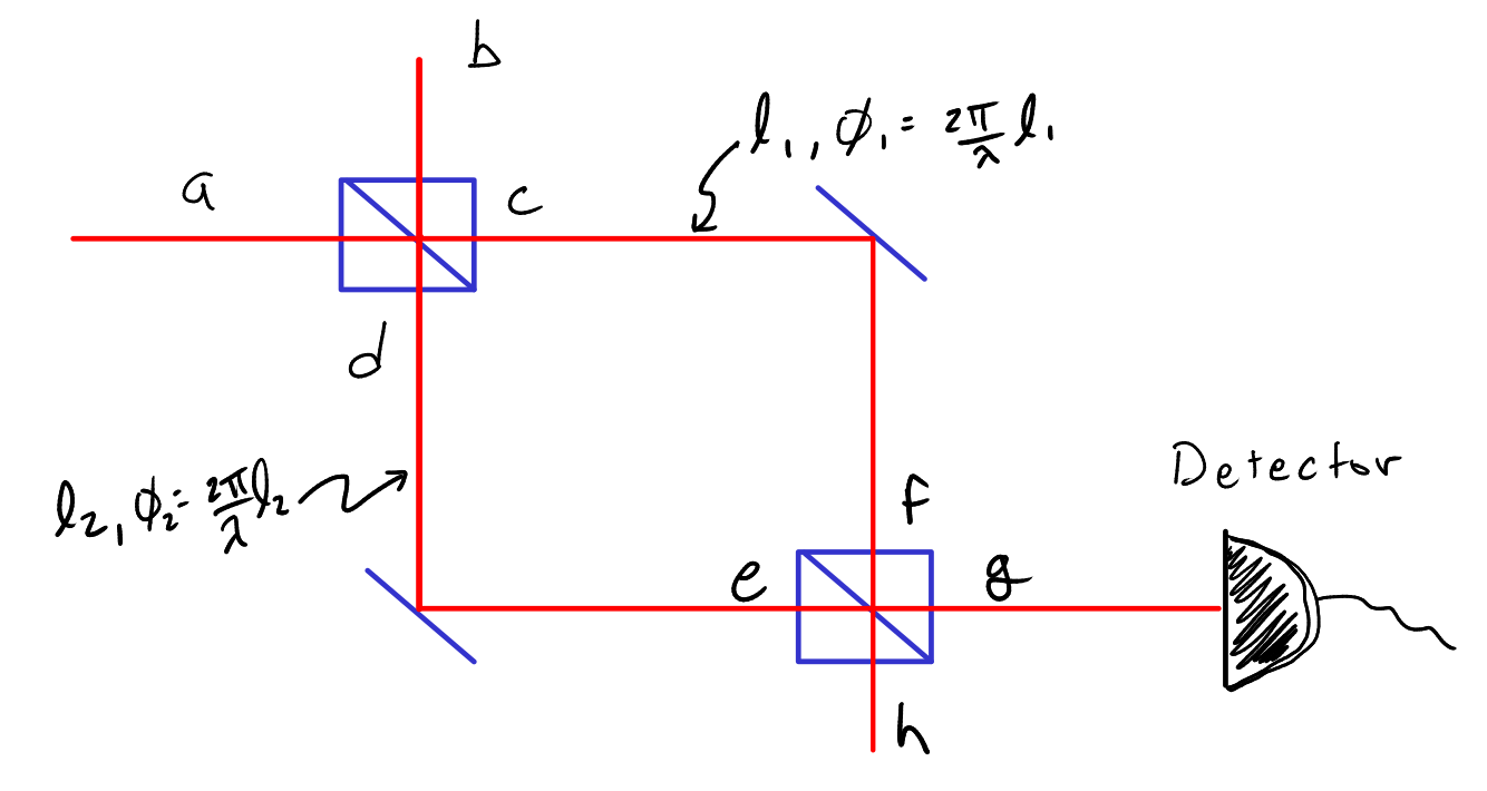
Fig. 28 Considering all inputs and outputs for the complete description of the Mach-Zender interferometer.

Now we can proceed to find the annihilation operators as before, but with all inputs included.

\[\chat = \frac{\ahat + \bhat}{\sqrt{2}}\]

and

\[\dhat = \frac{\ahat - \bhat}{\sqrt{2}}\mathrm{.}\]

We then account for propagation over paths \(l_1\) and \(l_2\) which lead to a phase shift of \(\phi_n = 2 \pi l_n/\lambda\).

\[\ehat = \dhat e^{i\phi_2}\]

and

\[\fhat = \chat e^{i\phi_1}\mathrm{.}\]

From here, we account for the fact that at the second beamsplitter we have

\[\ghat = \frac{\ehat + \fhat}{\sqrt{2}}\]

and

\[\hhat = \frac{\ehat - \fhat}{\sqrt{2}}\mathrm{.}\]

After substituting everything in we get the final expression for \(\ghat\):

\[\ghat = e^{i\phi_2} e^{i\Delta\phi/2} \bigg \lbrace \ahat \cos(\Delta\phi/2) + i \bhat \sin(\Delta\phi/2) \bigg \rbrace \]

where \(\Delta \phi = \phi_1 - \phi_2\), the phase difference between the two arms.

Note that the number operator for \(g\) is then:

\[\gdagger \ghat = \cos^2(\Delta \phi /2)\adagger\ahat + j\adagger\bhat \cos(\Delta\phi/2)\sin(\Delta\phi/2) - j\bdagger\ahat \cos(\Delta\phi/2)\sin(\Delta\phi/2) + \bdagger\bhat \sin^2(\Delta\phi/2) \mathrm{.}\]

Given our input state is \(\ket{1}_a \ket{0}_b\), the photon number is then found by taking:

\[N_g = \bra{0}_b \bra{1}_a \gdagger \ghat \ket{1}_a \ket{0}_b = \frac{1}{2} \lbrace 1 + \cos(\Delta\phi ) \rbrace \mathrm{.}\]

Note that only the terms with \(\adagger \ahat\) have a non-zero contribution – this justifies our neglecting the vacuum-state inputs for calculation of the output photon number.

However, it we emphasize that you must use this more complete treatment and account for the vacuum-state inputs to accurately predict the quantum noise in systems. For example, the standard deviation of the photon number depends on \(\hat{N}^2\) (see the note in Mean and Standard Deviation Observables), and the vacuum state inputs can contribute to the expectation \(\left < \hat{N}^2 \right >\). As a further example, to see the importance of the vacuum state input in interferometry, please see the use of squeezed vacuum to reduce quantum noise as described in EXTRAS – Homodyne Detection.

Accounting for the partial absorber

For the partial absorber, again our treatment in the text was adequate for accounting for the outgoing photon number. However, a rigorous solution requires accounting for the vacuum state here again.

The partial absorber can in fact be modeled as a beamsplitter with adjustable transmission/reflection with one input being the vacuum state, the other being the input state, and one output going to a perfect absorber, and the other transmitting out. See Fig. 29.

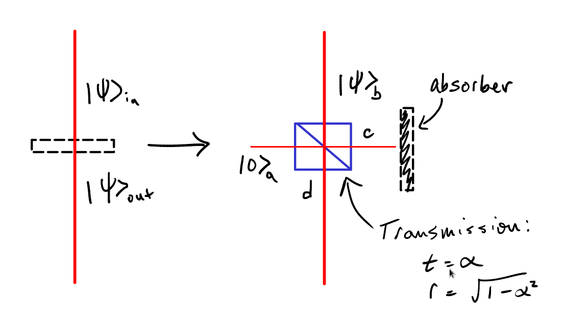
Fig. 29 Model of a partial absorber using a beamsplitter to account for the vacuum state.

This model accounts for the vacuum state properly. Note here the beamsplitter is not a 50:50 beamsplitter to account for the adjustable transmission probability. The input/output relations are similar, with:

\[\chat = t\ahat + r\bhat\]

and

\[\dhat = r\ahat - t\bhat \mathrm{.}\]

From the derivation in the text, we have that \(t = \alpha\), and \(r = \sqrt{1 - \alpha^2}\). You can show that with this element in the Mach-Zender interferometer, the output photon number expectation is equivalent to what we derived, with the number of detected photons being

\[N_d = \frac{1}{4}\lbrace 1 + t^2 + 2t\cos(\Delta \phi)\rbrace \mathrm{.}\]

However, as noted earlier, the impact of this absorbing object is to effectively couple in vacuum state which must be accounted for during analysis of the quantum noise limit of the interferometer.

Accounting for Bandwidth

Finally, let us address the issue of the state having a non-zero bandwidth. Up until now, we have discussed states from the context of a single frequency. Our results would imply that interference would continue indefinitely as one changes delay. However, in practice our source states will have a non-zero bandwidth which leads to a finite range of delays over which one would observe interference. In this section, we will introduce how to account for this bandwidth.

For the case of a non-zero bandwidth, we can write our single-photon input state as

\[ \ket{\psi_\mathrm{in}} = \int_{-\infty}^\infty \mathrm{d}\omega \phi(\omega) \ket{1;\omega}_a \mathrm{,}\]

where \(\phi(\omega)\) contains the spectral amplitude and phase distirubtion for each frequency component. Note that by normalization we have that

\[\braket{\psi_\mathrm{in}}{\psi_\mathrm{in}} = \int_{-\infty}^\infty \mathrm{d}\omega_1 \int_{-\infty}^\infty \mathrm{d}\omega_2 \phi(\omega_2)^{*} \phi(\omega_1) \braket{1;\omega_2}{1;\omega_1}_a \]

Given orthonormality we have that \(\braket{1;\omega_2}{1;\omega_1}_a = \delta(\omega_2 - \omega_1)\), which removes the second integral, simplifying everything to

\[\braket{\psi_\mathrm{in}}{\psi_\mathrm{in}} = \int_{-\infty}^\infty \mathrm{d}\omega_1 |\phi(\omega_1)|^2 = 1\]

What is this all saying? Basically, we are saying that we have a probability of 1 of finding a photon over a range of frequncies defined by the distribution \(|\phi(\omega)|^2\). While we will always find a photon, we just don’t know for certain what energy it has due to the finite bandwidth of our source.

Taking this further, we can define the state in terms of the creation operator.

\[ \ket{\psi_\mathrm{in}} = \int_{-\infty}^\infty \mathrm{d}\omega \phi(\omega) \adagger(\omega) \ket{0}_a \mathrm{.}\]

In this way, we can track the operators through any system in the same way as we already have for the single-frequency states. Following this method, we can re-express our output state calculated from our earlier analysis of the interferometer now accounting for the non-zero bandwidth:

\[\ket{\psi_\mathrm{out}} = \int_{-\infty}^\infty \mathrm{d}\omega \cos \bigg ( \frac{\omega \Delta l}{2c} \bigg )\phi(\omega) \ket{1;\omega}_a \mathrm{.}\]

Note that here it is important as we write the phase difference in terms of \(\omega\) and the path length difference \(\Delta l\). What is the probability of finding a photon then. Well, we just take \(\braket{\psi_\mathrm{out}}{\psi_\mathrm{out}}\), which becomes

\[\braket{\psi_\mathrm{out}}{\psi_\mathrm{out}} = \int_{-\infty}^\infty \mathrm{d}\omega_1 \int_{-\infty}^\infty \mathrm{d}\omega_2 \phi(\omega_2)^{*} \phi(\omega_1) \cos \bigg ( \frac{\omega_1 \Delta l}{2c} \bigg )\cos \bigg ( \frac{\omega_2 \Delta l}{2c} \bigg )\braket{1;\omega_2}{1;\omega_1}_a \]

Again, we have that \(\braket{1;\omega_2}{1;\omega_1}_a = \delta(\omega_2 - \omega_1)\), and after substitution this again gets us back to one integral:

\[\braket{\psi_\mathrm{out}}{\psi_\mathrm{out}} = \int_{-\infty}^\infty \mathrm{d}\omega_1 |\phi(\omega_1)|^2 \cos \bigg ( \frac{\omega_1 \Delta l}{2c} \bigg )^2 \mathrm{.}\]

Note that the major difference here is the adddition of the cosine term. This resuts in an oscillation of the output photon detction probability. Note that the bandwidth probability distirubution function \(\phi\) then dictates the range of delays over which you see this oscillation in probability. Importantly, note that that all phase information inside of \(\phi\) is lost as the output is dictated by \(|\phi|^2\) (our interferometer is, after all, only sensitive the phase differences between the two arms, and not to the absolute phase of the incoming state).

Let’s now numerically explore the single-photon interference accounting for bandwidth.

We start by taking a Gaussian distribution for \(\phi\).

import numpy as np
import matplotlib.pyplot as plt

# -- Settings -- 
c  = 300 #speed of light in nm/fs
lambda_0 = 810 # central wavelength in nm
sigma = 0.3 # bandwidth of the photons in petahertz
omega_0 = 2*np.pi*c/lambda_0 #central frequency of the photons

# -- Calculations

#Set up the frequency axis (rad/fs)
omega = np.linspace(omega_0 - 10*sigma, omega_0 + 10*sigma, 10000)

#Define the initial gaussian frequency distribution
phi = np.exp(-(omega - omega_0)**2/sigma**2)

#Ensure it is normalized properly
norm_factor = np.sqrt(np.trapz(np.abs(phi)**2, x = omega))
phi = phi/norm_factor

#Plot for visualization
fig = plt.figure()
plt.plot(omega, abs(phi)**2, label=r'$\phi(\omega)$')
plt.legend(fontsize=13)
plt.xlabel(r'$\omega$ (rad/fs)', fontsize=13)
plt.ylabel(r'$\phi(\omega)$', fontsize=13);

fig.set_size_inches(10, 7)

Show code cell output Hide code cell output

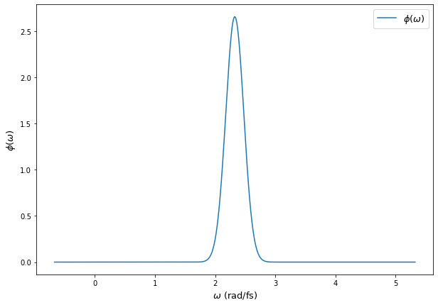
Fig. 30 Normalized spectral distribution of single-photons.

Next, we define the path length difference and perform the integral for each choice of delay.

#-- Settings -- 

#Define the delay length (in nm)
l = np.linspace(-10e3, 10e3, 1000) #Path length difference to scan over

# -- Calculations -- 

#Set up vector for output probabilities
P_out = np.zeros(l.shape) #Probability of seeing a photon at the output

#Now calculate output probability for each delay
for cc in range(0, l.size):

    P_out[cc] = np.trapz(np.abs(phi)**2*np.cos(omega*l[cc]/2/c)**2, x = omega)

fig = plt.figure()
plt.plot(l, P_out)
plt.xlabel('delay length (nm)', fontsize=13)
plt.ylabel('photon detection probability', fontsize=13);

fig.set_size_inches(10, 7)

Show code cell output Hide code cell output

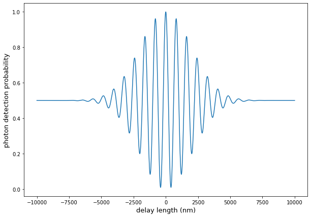
Fig. 31 Single-photon interference as a funciton of delay with finite bandwidth.